Mass Flow meter¶

There was one experiment in which air mass flow rate had to be measured in a pipe. The challenge was that air was not pure, it contained tracer particles used for Particle Image Velocimetry. There are multiple ways to measure the mass flow rate through the pipe, but we were searching for some inexpensive solution to the problem. The immediate solution at hand was to use the Rotameter, shown in below figure.

Rotameter

Rotameter principle¶

Rotameter is the variable area flow meter. When fluid flows through the rotameter, it has to first lift the float that is fixed inside the rotameter. The lift of the float is in direct relationship with the velocity. The cross-sectional area is also known at the height of float. Hence flow rate can be determined.

Rotameters gives the output in volumetric flow rates. i.e. Liters per minute (LPM) or $m^3/s$. But for the task at hand, mass flow rate of the air was required.

Converting $m^3/s$ to $kg/s$¶

To convert the obtained volumentric flow rate($m^3/s$) from rotameter into mass flow rate($kg/s$), density of the flow is required. If we know the density of the flow at any point on the flow path of rotameter then we can convert volumetric flow rate into mass flow rate. This can be stated in another way,

$$ \dot{q} = Av$$$$ \dot{m} = \rho Av$$

If we know the density of the flow then we can convert the volumetric flow rate obtained from rotameter into mass flow rate. To get the density of the flow, we need to know the pressure of the flow. Hence, If we use the pressure measuring device before rotameter then we can get the estimate of the density of the flow.

rotameter setup
Rotameter with Pressure transducer attached before it

Above figure shows the setup of the rotameter, where pressure transducer (PT) is attached before rotameter. The pressure obtained from this PT will be indicative of the density of the flow. Hence using the rotameter LPM reading and PT reading in bars, we will be able to calculate mass flow rate in $kg/s$.

Use of ML¶

One way to convert the measured PT and LPM data into $kg/s$ is from theoretical approach. But then, we will also have to consider various losses of pipelines and connectors into account, whose values we don't know. But, we know this for sure that, with rotameter and PT value we can get mass flow rate. Hence, converting of the input values to output values was performed by ML-regression task. To perform ML, we first need the known value of mass flow rate and then characterize the rotameter setup using that. In short, we were required to calibrate the system. We used Alicat series mass flow controllers to supply known amount of mass flow rate $kg/s$ into the system and measure rotameter (LPM) and PT's (bar) value. Alicat mass flow controllers provide the mass flow rate in Standard Liters per Minute(SLPM) unit. Hence, the data shown below will showl SLPM as the unit of mass flow rate.

rotameter reading
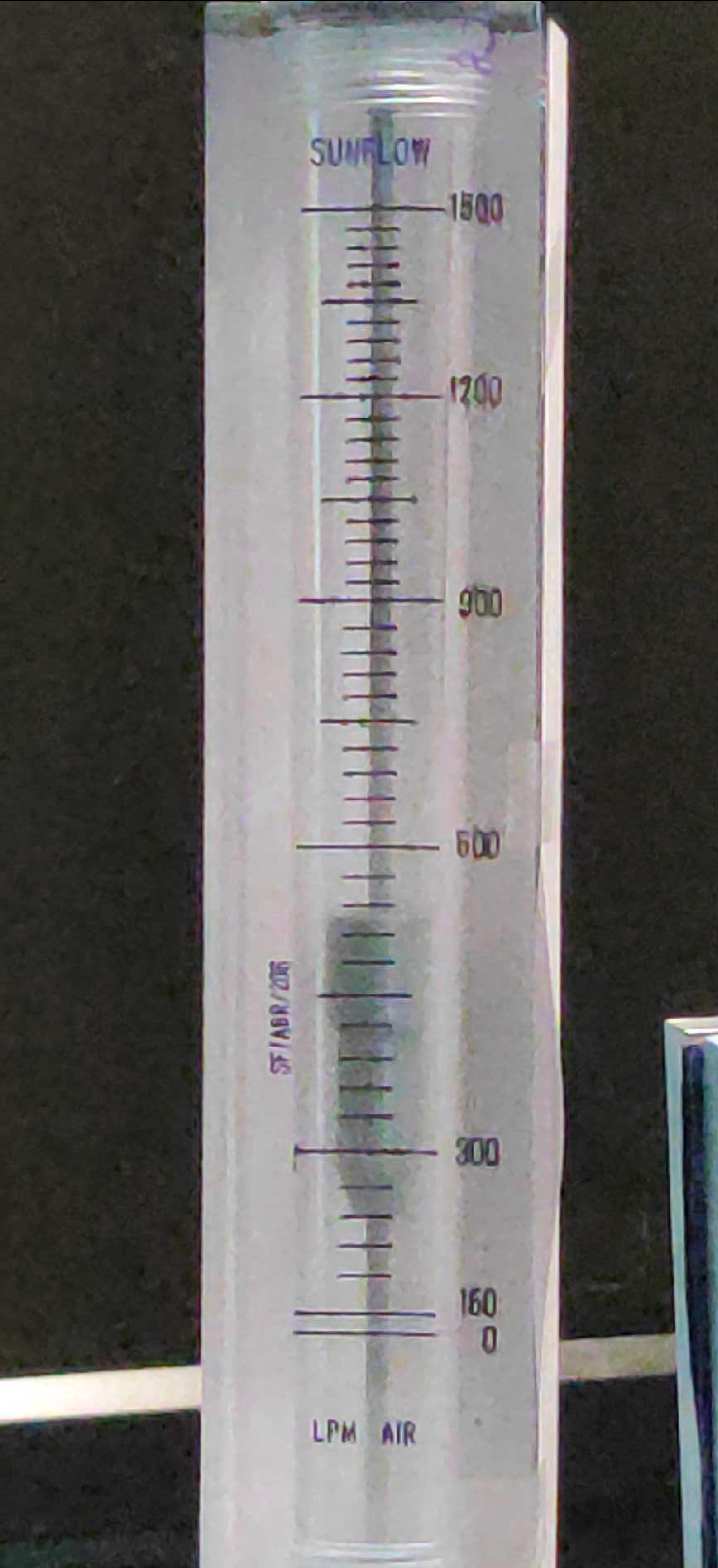
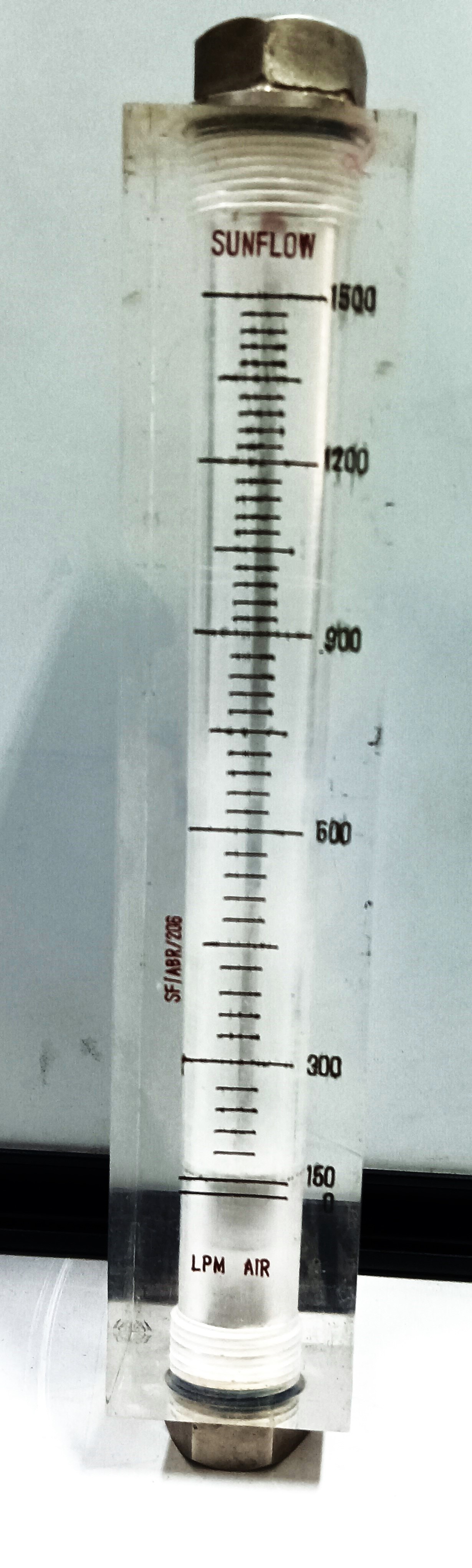
Reading of rotameter at one of the sample point

Below figure shows the plot of sample data collected during callibration of rotameter. It is observed that with increase in inlet pressure, the LPM reading of rotameter decreases for constant inlet SLPM. This is obvious, as we increase the inlet pressure, there will be increase in density of the flow, hence for a given inlet mass flow rate($\dot{m}$) the volumetric flow rate will reduce with increase in inlet flow density.

Fitting ML¶

We will split the sample data into 2 parts:- train and test data. The good practice is to divide the data into 3 parts:- train ,validation and test. But, here after the model fitting, the test was conducted on live data. Meaning, the model had to predict the mass flow rate[SLPM] through the pipe from given rotameter[LPM]reading and pressure[bar] reading, in real time. Hence, the full data was only split into two halves. 80% of the data was considered for training and 20% was reserved for testing purpose.

Errors in Train and Test data
------------------------------
{'root_mean_sq_err_train': 7.241, 'mean_abs_err_train': 5.889, 'root_mean_sq_err_test': 10.606, 'mean_abs_err_test': 8.626}
------------------------------
As above data shows, there is error of around 10.6 SLPM in prediction for data

 Model
------------------------------

Out[2]:

Pipeline(steps=[('poly_features',
                 PolynomialFeatures(degree=3, include_bias=False)),
                ('std_scaler', StandardScaler()),
                ('lin_reg', LinearRegression())])

In a Jupyter environment, please rerun this cell to show the HTML representation or trust the notebook.
On GitHub, the HTML representation is unable to render, please try loading this page with nbviewer.org.

The model was checked with real time data and the error was found to be within the desired range.

This shows that, using ML regression techniques, we can bypass the theoretical approach to calibrate the flow device. Although, this is not the standard way of acheiving the calibration. But, given the limitation of time and cost, the ML regression techniques can prove very helpful in such physical systems.

Thank you